Digital Filter Design in 30 minutes

Lately, I'm re-introducing myself to digital signal processing after the course I took in university. Back in the days, I performed really badly and even passed the course with a grade just above the threshold. Don't get me wrong, I loved the topic and its real-life applications. However, due to errands in my life, it became really hard to study for the course.

Two weeks ago, I decided to learn it again. Thanks to all the free time I have now, with AI-guided learning, I can learn it as fast as I can, with a focus on a real-life problem to understand the edge cases in use. Therefore, I started to implement a digital signal processing library in a programming language from scratch. Function generators, FFTs/iFFTs, windowing, plotting functions, etc., are already done, and the next step was to realise a digital filter. I asked for a resource on Reddit for a short and "enough" to understand the basics. The ones suggested weren't that great. Then, I did a guided learning session with LLMs, experiment what I learned using scipy in Python and said why not make the resource myself for the future learners.

This guide will be a story-like introduction to digital filter design. I write it for an audience that has minimal background in signal analysis.

Signals and Their Representation

I'm a simple guy, and for me, a signal is an information flow that changes over time or in any other medium. A sound, an image, a video, all of them are signals in my perception. From time to time, we need to modify the signals, either to reduce the noise or apply cool guitar effects. This is where signal processing experts come in and try to achieve the optimal system for their problem.

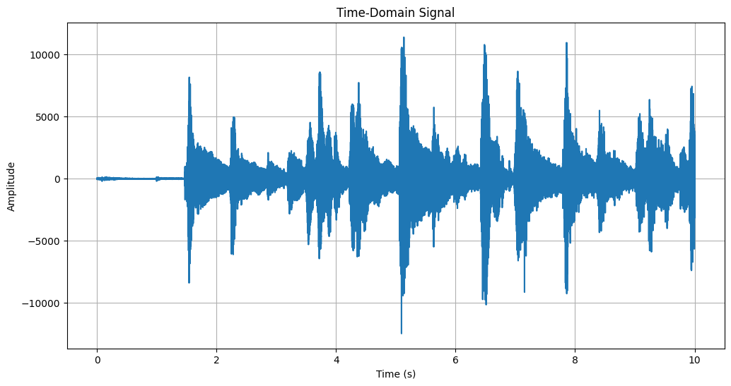
A analgoue signal is a continuous wave, which means it has no "samples" and has infinite resolution. However, in the computation domain, we are required to have samples since we can not store an infinite number of data points. We select a sample rate to only store a dedicated number of samples per second.

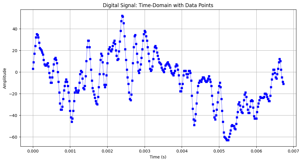
In the figure above, you can see what a digital signal actually looks like. Only the samples are stored, and the non-stored ranges are calculated using interpolation. When we have a high number of samples per second, it's easy to construct the continuous signal back using interpolation. However, this is not the case most of the time. For a set of data points, we can have a different signal reconstruction. Find an example below where we have three samples, and three waves can be constructed.

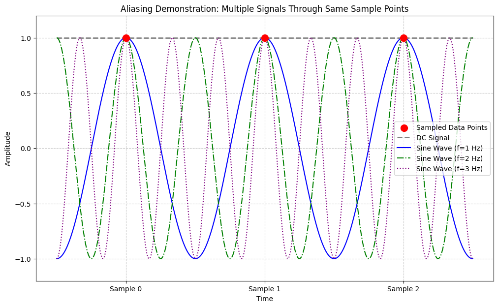
This is called aliasing. It is the problem of reconstructing N samples to correct continues wave. Luckily, we know how to solve it perfectly – at least up to a level. There's a Nyquist rate definition, and it says that a signal can be constructed perfectly if the highest frequency in the signal composition is below half of the sample rate.

So, for a sound signal (which is nearly always 44100 samples in our daily life), we can use the Nyquist rate and say that we can construct the signal from data samples for frequencies from 0 Hz to 22050 Hz.

One may ask, "What does it mean to have frequencies in a signal? Isn't it all random? Where do we see the periods?". Let's answer this question in the next section.

Frequency Domain

Normally, we express a signal in the time domain. Where a signal $y(t)$s values are dependent on $t$, a time variable. Although this is more intuitive for a general audience, the disadvantage is that it hides patterns of a signal.

A signal, even though it looks random, can be expressed using its patterns. Let's look at an example. Imagine having three sine signals with different frequencies. When we add their $y_n(t)$ values for every $t$, we'll see a signal that is a combination of all three and follows their characteristics. Find an example in the figure below.

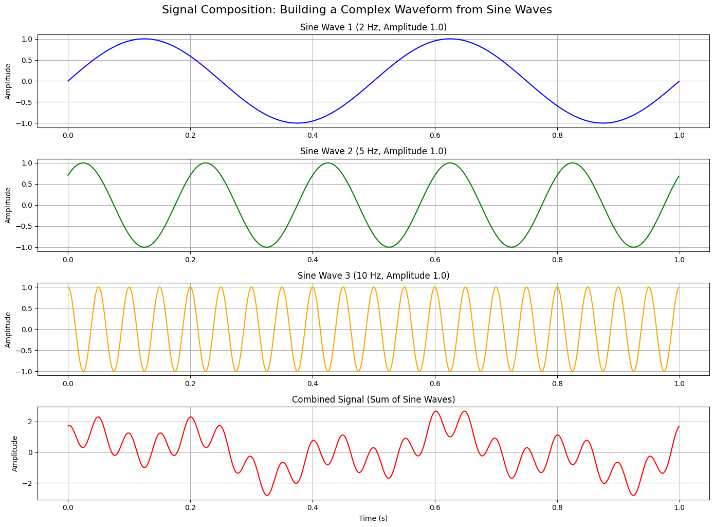
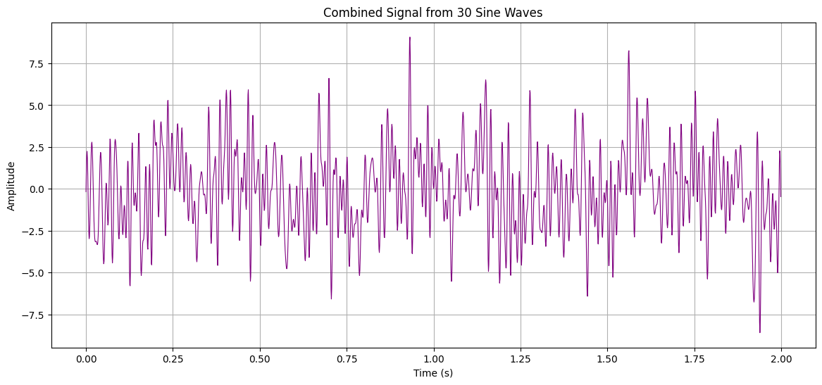
As you can see from the last figure's last plot, although a signal looks kinda random, it has periodic signals, or in my call, patterns inside. I know that some of you would still find the last one an easy-to-say example. Therefore, I generated the following figure, which is the combination of 30 perfect sine waves. If someone would show me this figure, I'd definitely say that it's all random!

Back in time, Fourier found a way to decompose a random-looking signal into its patterns. It's called the Fourier Transform. It gets a function $f(t)$ and converts it to $F(w)$ where $w$ is the angular frequency (radians/second). Although the equation is super important, for the sake of the current getting-started vibe, I'm not going to go into the depths of the equation. Please find this website for more details.

Fourier Transform (from time domain to frequency domain):

$$
F(\omega) = \int_{-\infty}^{\infty} f(t) e^{-j\omega t} dt
$$

Inverse Fourier Transform (from frequency domain to time domain):

$$
f(t) = \frac{1}{2\pi} \int_{-\infty}^{\infty} F(\omega) e^{j\omega t} d\omega
$$

By using the Fourier Transform on a quite random-looking signal, for example, the figure above with 30 frequencies, we can gather the frequency elements one by one with their phase and amplitude information. This is quite useful for signal processing, since we're mainly interested in a range of frequencies, and others can be ignored.

Imagine you capture a voice memo from your class. However, after you listened to the recording, you realised that there's a constant background noise. What you want to do is to cancel this noise somehow without touching the professor's voice. First of all, you'll apply the Fourier Transform to the recording to see what frequencies are there and at high amplitude. Then, you're going to find the frequency range your professor speaks – this will be mainly experimentation with different frequencies and listening to them. When you find that your professor's voice is between $[f_1, f_2]$ Hz, you're going to remove all other frequency components in the Fourier Transform's output, which are $(0, f_1)$ and $(f_2, \infty)$. When you have the sine wave composition for the frequencies only between $f_1$ and $f_2$, you'll apply the Inverse Fourier Transform to get the time domain back, and listen to a recording that has no environmental noise! This is actually a simple explanation of how an equaliser works.

As you see, what Fourier achieves is quite remarkable. That's why it's also selected as one of the most important 10 equations by an IEEE journal that I cannot recall now. In signal processing, we can work with any domain we think is best, and frequency is one of the most popular ones for many problems.

In the digital domain, we cannot calculate the integrals for a continuous signal. Therefore, there was a need to modify the original Fourier Transform to work with discrete/digital samples. In the following equations, you can see the modified version. The logic and the background are all the same, but this one is more useful for us in digital signal processing. Please find this nice chapter from Oppenheim's Signals and Systems textbook on how to derive the discrete-time from the original equation.

Discrete-Time Fourier Transform (from time domain to frequency domain):

$$
X(\omega) = \sum_{n=-\infty}^{\infty} x[n] e^{-j\omega n}
$$

Inverse Discrete-Time Fourier Transform (from frequency domain to time domain):

$$
x[n] = \frac{1}{2\pi} \int_{-\pi}^{\pi} X(\omega) e^{j\omega n} d\omega
$$

Z-Transform

The problem with the Fourier Transform is its nature, which only allows us to use it for well-behaved signals. You can use it for stable signals (do not expand to infinity in amplitude) or non-causal ones (no start or end time of the signal). As you can see, it is useful for a specific part of the world; however, the world is not that simple.

In real life, our signals have a starting point. From time to time, we see them being amplified to infinity. Nothing is perfect, and we need to have a function to generate the frequency domain for these signals as well.

Here's the generalised version of the (Discrete-Time) Fourier Transform. It is called the Z-transform.

$$
X(z) = \sum_{n=-\infty}^{\infty} x[n] z^{-n}
$$

where $z = re^{j\omega}$. Let's substitute the z with its definition to see what it looks like using $\omega$

$$
X(e^{j\omega}) = \sum_{n=-\infty}^{\infty} x[n] (re^{j\omega})^{-n}
$$

Please notice the difference between the Discrete-Time Fourier Transform and the Z-Transform. It is the only $r$ multiplier factor. This is called the damping factor. It tells us if this frequency will stay the same ($r=1$), grow to infinity ($r>1$) or decay to zero ($r<1$).

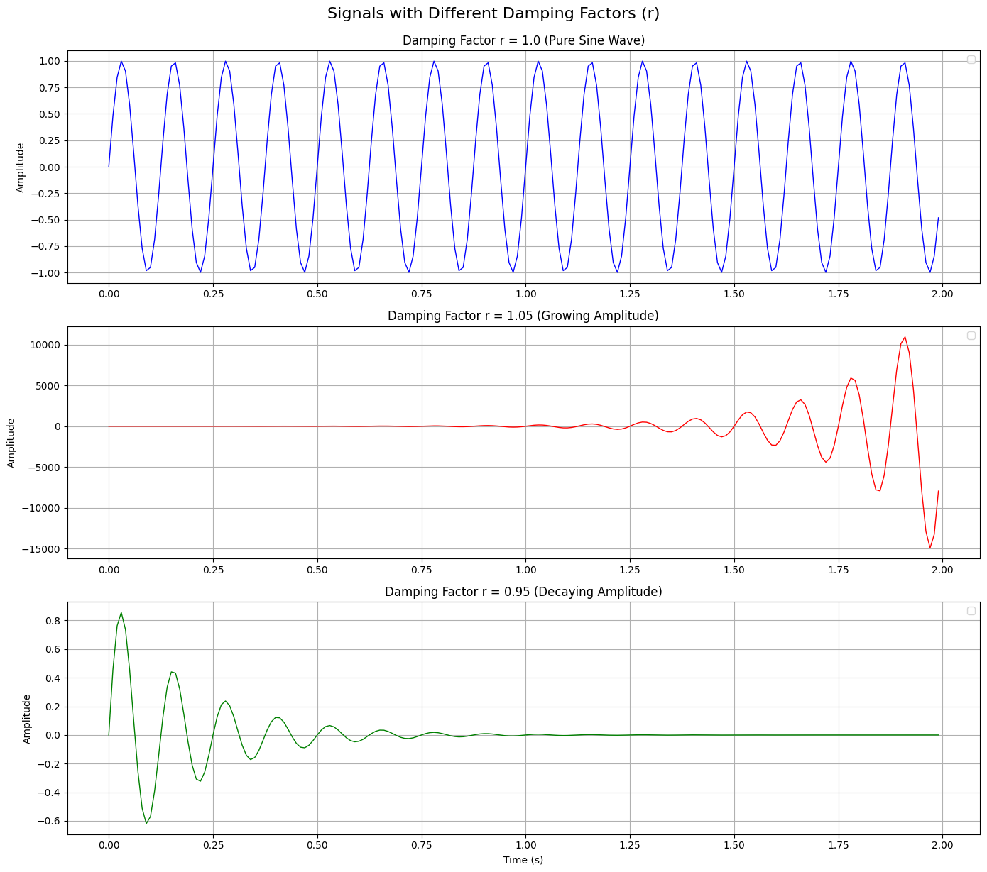
As you can suspect, the Fourier Transform is the special case of the Z-Transform for $r=1$, and that's why we cannot use it for signals decaying or growing.

The best part of the Z-Transform is to easily describes the time delays with a power of $z$. It's called the time shifting property, and through the guide, we'll use this property to express the delays in our signals.

Let's imagine shifting our sample by $k$,

$$
Y_{n}(z) = \sum_{n=-\infty}^{\infty} x[n-k] z^{-n}
$$

To simplify this, we perform a change of variables. Let $m=n−k$, which implies $n=m+k$. As $n$ goes from $−\infty$ to $\infty$, $m$ does as well.

$$
Y_{n}(z) = \sum_{m=-\infty}^{\infty} x[m] z^{-(m+k)}
$$

We can pull the constant $z^{−k}$ out of the summation because it does not depend on $m$:

$$
Y_{n}(z) = z^{-k} \sum_{m=-\infty}^{\infty} x[m] z^{-m}
$$

As we already defined the summation part as the Z-transform of a signal, we can substitute our $Y_{n-k}(z)$ there.

$$
Y_{n}(z) = z^{-k} Y_{n-k}(z)
$$

This derivation proves to us that a signal shifted by $k$ samples to the back (due to the minus), in Z-domain, corresponds to a multiplication with $z^{-k}$. We'll use this property in the next section to provide a foundation for how we can write a signal $Y(z)$ based on the inputs and outputs of a system.

Transfer Function of a System

Every system is a black box. There are inputs and output pairs, and a mapping from inputs to outputs. This mapping can be a polynomial, a differential equation, a machine, a web form, a neural network, or a super-weird alien technology. Most of the time, we design our systems based on the requirements that define the inputs we can get and the outputs we should produce. This is called model-driven design.

When a model-driven design is completed, the system is given to an engineer with field information. For example, a model that converts 12 Volts to 5 Volts is given to electrical engineers, and they realise the model within a circuit design. Another example, a model that suppresses particular vibrations in a machine is given to a mechanical engineer, and they realise the model within correct material selection and mechanical placements. This is how I tend to work in my software design process as well. I know which inputs are given to me, and what outputs are expected from them, and prepare an algorithm that will realise it in your device.

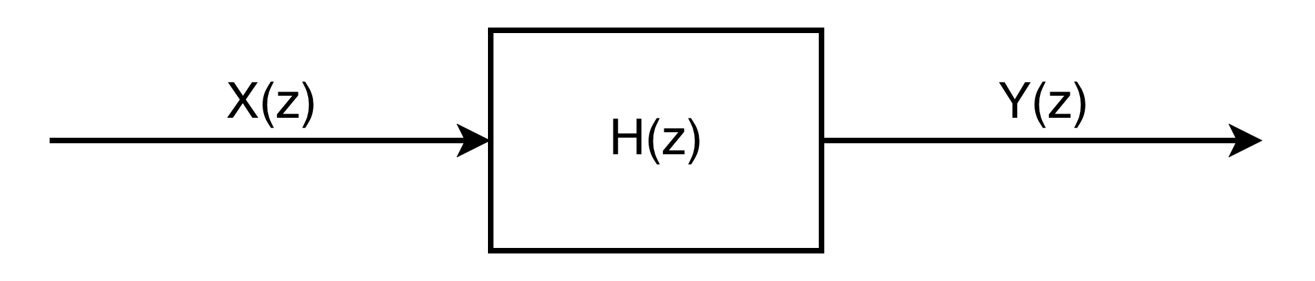
Therefore, until the white box is solved (this is how QA engineers call a system where the inner logic is known), we have to find a mapping for our black box. This mapping is called a transfer function (or system function), and is defined as the ratio of outputs to inputs in complex variables.

Discrete-Time Transfer Function

$$
H(z) = \frac{Y(z)}{X(z)}
$$

It's continues-time form is constructed with the Laplace Transform, which is not in the scope of the current guide.

The best part of the transfer functions is their ability to cascade. It means that one can place $H_1(z)$, $H_2(z)$, $H_3(z)$, and many more next to each other where each ones outptus will be an input to the next one to represent a high-order system.

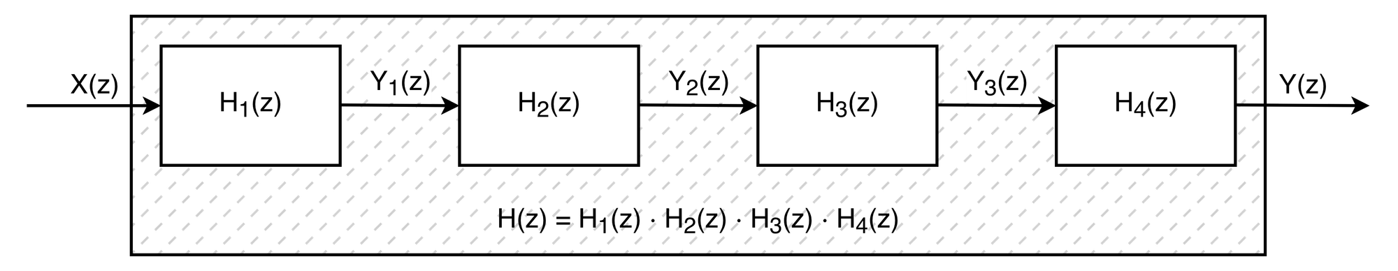
As you can see from the figure above, we can express a really complex transfer function with high-order components as a cascaded individual system, with simple equations.

For the digital signal case, we try to imagine the most general block-box system and try to find its transfer function. First of all, an output discrete signal $y[n]$ will be dependent on a discrete input $x[n]$.

$$
y[n] = b_0 \cdot x[n]
$$

It is also possible that $y[n]$ is dependent on its previous input $x[n-1]$, which is called feedforward, or on previous ones.

$$
y[n] = b_0 \cdot x[n] + b_1 \cdot x[n-1] + b_2 \cdot x[n-2] + b_3 \cdot x[n-3] + \text{...}
$$

It is also possible that $y[n]$ is dependent on its previous outputs $y[n-1]$, which is called feedback, or on previous ones.

$$
y[n] = \sum_{\alpha = 0}^{n} b_\alpha \cdot x[n-\alpha] + \sum_{\beta = 0}^{n-1} a_\beta \cdot y[n-\beta]
$$

It's also possible that $y[n]$ can have a scalar factor. Let's collect $y[n-\beta]$s to the left and $x[n-\alpha]$s to the right. We don't need to care about the coefficient's sign since we describe them for our ease.

$$
\sum_{\beta = 0}^{n} a_\beta \cdot y[n-\beta] = \sum_{\alpha = 0}^{n} b_\alpha \cdot x[n-\alpha]
$$

This is the most general equation we can have for a digital signal system. To find a transfer function as the ratio of outputs to inputs, we need to find a way to express all of the outputs in one output variable and all of the inputs in one input variable. Luckily, this is what we can do with the Z-transform, and its time shifting property!

Let me remind you of the Z-transform of the basic input and output to show how they can help us to unify everything into $Y(z)$ and $X(z)$.

$$
\mathcal{Z}\{x[n-\alpha]\} = z^{-\alpha}X(z)
$$

$$
\mathcal{Z}\{y[n-\beta]\} = z^{-\beta}Y(z)
$$

Let's apply the Z-transform to the all system equation.

$$
\sum_{\beta = 0}^{n} a_\beta \cdot z^{-\beta}Y(z) = \sum_{\alpha = 0}^{n} b_\alpha \cdot z^{-\alpha}X(z)
$$

Since a transfer function is defined as $H(z) = Y(z) / X(z)$, we can reorganise the equation and find the transfer function of a digital signal system.

$$
H(z) = \frac{Y(z)}{X(z)} = \frac{\sum_{\alpha = 0}^{n} b_\alpha \cdot z^{-\alpha}}{\sum_{\beta = 0}^{n} a_\beta \cdot z^{-\beta}}
$$

The form that most of us see in the textbooks is as follows. It is clearer to express it this way since there's no more $\alpha$ and $\beta$ magic.

$$
H(z) = \frac{Y(z)}{X(z)} = \frac{b_0 \cdot z^{-0} + b_1 \cdot z^{-1} + b_2 \cdot z^{-2} + b_3 \cdot z^{-3} + \text{...}}{a_0 \cdot z^{-0} + a_1 \cdot z^{-1} + a_2 \cdot z^{-2} + a_3 \cdot z^{-3} + \text{...}}
$$

We derived the most important thing we'll use to design our filters. We'll use this equation to define a filter, and talk about what it tells us.

Basics of Digital Filters

Many define filters based on different aspects. I like to define them as any transfer function that is applied to a digital signal. This is why in the current section, we never talked about a filter. In the end, they are not special; just a simple black-box system where we know what we want to get as an output based on an input pair. The general transfer function we found in the previous section is a transfer function of a digital filter as well.

The coefficients of $Y(z)$ are known as $a$ coefficients, and $X(z)$ are b coefficients. One can design a filter based on only the coefficients since it can represent the system response as a combination of feedforward and feedback loops.

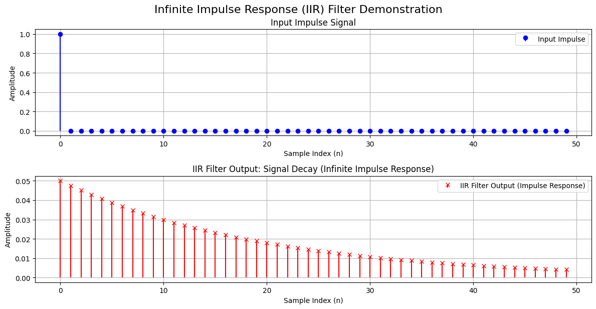
Feedback is to change the current output based on the previous output. In time-domain representation, it means that $y[n]$ is affected by $y[n-1]$. We represented it with $a$-coefficients. The roots of a feedback are called poles. Because the filter feeds its own previous calculations back into itself to create the new one, its response to an impulse can mathematically ring out forever, creating
an Infinite Impulse Response (IIR).

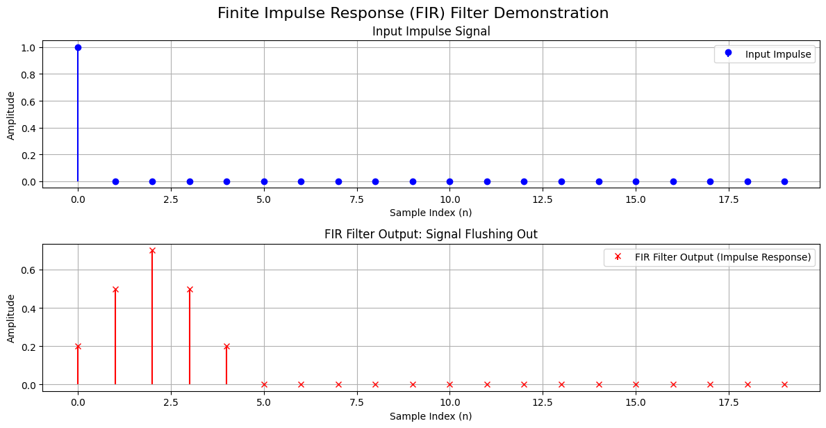
Feedforward is to change the current output based on previous inputs. In time-domain representation, it means that $y[n]$ is affected by $x[n]$, $x[n-1]$, etc. We represented it with $b$-coefficients. The roots of a feedforward are called zeros. If a filter only uses $b$ coefficients, it has a Finite Impulse Response (FIR) because the signal eventually flushes out of the system.

Poles and Zeros

The poles and zeros are quite important since they define the nature of our filter and its output behaviour. Zeros are the roots of the numerator, and poles are the roots of the denominator.

Before trying to understand what zeros and poles do to our input and output mapping, let me remind you what information the $z$ variable holds. It is an alias defined as $z = re^{j\omega}$ as we discussed earlier. The $r$ variable holds the dumping factor, which tells us if our signal will be zeroed out, grow, or stay as is. $\omega$ is the angular frequency in radians per second, which is defined as $\omega = 2 \pi f / f_{sr}$ where $f$ is the frequency, and $f_{sr}$ is the sampling rate. Therefore $\omega$ variable holds the frequency component of the response. We are going to use this knowledge to understand how zeros and poles affect our output.

We know that the numerator of any ratio can be zero, which results in the output being 0 as well. This means that the frequencies in a filter that make the numerator zero, the filter will zero out/cancel them. It is not important what dumping factor we have; the frequency will be zero-out.

On the other hand, mathematically, it is not possible to have a ratio divided by zero. We can only approach zero in the denominator using a limit, which results in our ratio's result going to infinity. This is true in the case of a filter's poles as well. The frequencies that make our denominator zero might cause the filter to have an unstable response, depending on the dumping factor. For a dumping factor $r > 1$, the filter will generate a response that grows indefinitely, and cause the system to be burned and smell bad. If the dumping factor is exactly 1, $r = 1$, we can still conclude that the system will be unstable since the previous consistent output will be added to the next output in a feedback loop, and it will generate an unstable system where the output grows to infinity. Again, the same bad smell. On the other hand, for any dumping factor $r < 1$, the system is considered stable since the response will be zero out eventually.

So, in a summary,

• Zeros are the roots that reduce the signal of a frequency and eventually zero outs them.
• Poles are the roots that increase the signal of a frequency and eventually goes infinity if $r \geq 1$.

One can calculate zeros and poles for any filter design to understand its stability by solving for the variable $z = r e^{j\omega} = r e^{j 2 \pi f / f_{sr}}$ for the equations below.

$$
\text{Zeros} \rightarrow b_0 \cdot z^{-0} + b_1 \cdot z^{-1} + b_2 \cdot z^{-2} + b_3 \cdot z^{-3} + \text{...} = 0
$$

$$
\text{Poles} \rightarrow a_0 \cdot z^{-0} + a_1 \cdot z^{-1} + a_2 \cdot z^{-2} + a_3 \cdot z^{-3} + \text{...} = 0
$$

It is important to note that we want our systems to be causal, which means that our system should be only dependent on the previous values and not future ones. When a transfer function where the degree of the numerator was higher than the denominator, without a corresponding delay, it would be trying to calculate an output using a future input. Therefore, we need to make sure that we have the same number of poles and zeros (roots of the numerator and denominator).

It can be easily realised by placing poles at $z = 0$, which won't have any effect on the system's amplitude response but cause a time delay, which is what we want to not be dependent on future values. On the other hand, we do not need to place zeros at infinity explicitly to match the number of poles since the nature of the equation introduces them implicitly.

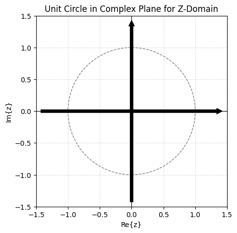
Unit Circle

We can use a complex plane where the vertical axis shows the imaginary part and the horizontal axis shows the real part of the $z$ variable. The poles and zeros can be placed into this plane to visualise their stability easily. Furthermore, we can have a unit circle on $|z| = 1$ to indicate the dumping factor effect of IIR filters.

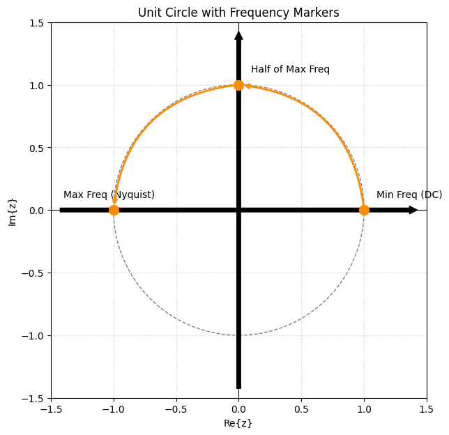
Within this plane, we can place our zeros and poles within a distance to the origin of $r$ (in the $z$). First of all, the signal's frequency is encoded on the $Re\{z\}$ axis, where 0 degrees (or 0 radians) represents the lowest frequency at $(1, 0)$, and 180 degrees (or $\pi$ radians) represents the highest frequency at $(-1, 0)$.

One can calculate it using $z = r e^{j 2 \pi f / f_{sr}}$ and inserting the values into the equation for the highest frequency (based on the Nyquist rate). I'll set $r = 1$ to only consider one type of dumping, the steady-state one, but this can be applied to all other $r$s.

$$
z = r \cdot e^{j 2 \pi f / f_{sr}} = 1 \cdot e^{j 2 \pi 22050 / 44100} = e^{j \pi} = -1
$$

The maximum frequency resides on $Re{z} = -1$ and $Im{z} = 0$. And with the lowest frequency, 0 Hz,

$$
z = r \cdot e^{j 2 \pi f / f_{sr}} = 1 \cdot e^{j 2 \pi 0 / 44100} = e^{0} = 1
$$

The minimum frequency resides on $Re{z} = 1$ and $Im{z} = 0$. Let's do it for half of the maximum frequency as well, to understand how it flows from max to min,

$$
z = r \cdot e^{j 2 \pi f / f_{sr}} = 1 \cdot e^{j 2 \pi 11025 / 44100} = e^{j 0.5} = +j
$$

The half of the maximum frequency resides on $Re{z} = 0$ and $Im{z} = -1$. That's perfect. It shows that the frequencies for the $r = 1$ case are like walking on the top half of a circle. For any other $r$, imagine the same walk, but with a circle of a different radius.

You may ask why we have the negative side of the imaginary plane. We will use that part to present complex conjugates of the roots on the top side, resulting in real numbers for $a$ and $b$ coefficients.

When designing a filter, the unit circle or the complex Z-plane is used to show the poles (with X) and zeros (with O) to understand the stability visually.

Filter Design

• Frequencies to Poles and Zeros Calculation
• Poles and Zeros to A and B coefficients
• Transfer function with A and B to Bode Plots

The design of a digital filter starts with gathering the requirements of the filter, such as what frequencies should be suppressed, what frequencies should be resonated (grow), and how steep we want the transitions to be, etc.

When all the requirements are set, we convert all the frequencies to the poles and zeros and plot them on the complex Z-plane (with unit circle) to see the stability of the system, and modify them if necessary. After the placement of poles and zeros is ready, the filter's frequency response is drawn with the x-axis as frequency on a logarithmic scale and the y-axis as amplitude in decibels. The same plot is drawn for the phase in the y-axis to understand the delay of the system – this is out of the scope for now. This plot is called a Bode plot and is quite useful to understand how our filter behaves.

I want to make some examples in this section to show you how we can design a filter from scratch – and as fast as possible. The filters will be low-pass, high-pass filters, a low-pass resonator, a notch filter, and a bandpass.

Low-Pass Filter

As the name suggests, it is a filter that only allows low frequencies to pass and blocks high frequencies. However, when a signal passes through a filter, the transition from "pass" to "block" isn't a sudden change. It is a gradual slope. Therefore, as engineers, we had to define a threshold that would indicate when the "cutoff" actually happens. Therefore, by the standards, we call this cutoff to happen on the exact point where the signal loses exactly half of its original energy/power. By the definition of decibels, we can calculate this point as $-3.01$ dB.

$$
10 \cdot \log_{10}(\frac{\text{Current Power}}{\text{Total Power}}) = 10 \cdot \log_{10}(\frac{\alpha}{2\alpha}) = 10 \cdot \log_{10}(0.5) = -3.01 \text{dB}
$$

Let's design the simplest low-pass filter first by adding a zero to the highest frequency, which is $z = -1$ in the unit circle. Please remember that we have to introduce a pole to have the same number of poles and zeros to make the system causal.

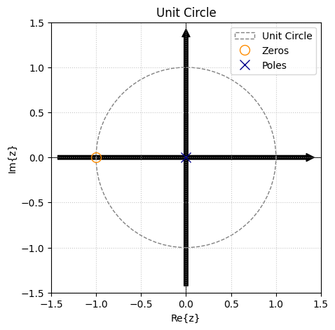
So, we have a zero at $z = -1$ and a pole at $z = 0$. It means that our transfer function has a first-order polynomial in its numerator and denominator.

$$
H(z) = \frac{z - z_0}{z - z_x} = \frac{z + 1}{z - 0}
$$

We want to express the transfer function in the form of delay shifts of $z^{-k}$, therefore, we are going to divide the terms by $z$ to find our $a$ and $b$ coefficients.

$$
H(z) = \frac{z + 1}{z} = \frac{1 + z^{-1}}{1 + 0 \cdot z^{-1}}
$$

We can see that our $a$ coefficients are $[1, 0]$ and $b$ coefficients are $[1, 1]$. This transition from zero-pole to transfer functions' $a$ and $b$ coefficients are easy for a few poles, but hard for many. Therefore, from now on, I'll use scipy's signal.zpk2tf function. It gets poles, zeros and a magnitude factor $k$ and outputs two arrays that are our transfer function's coefficients.

from scipy import signal

# Define your zeros and poles.
zeros = [-1.0]
poles = [0.0]

# Convert Zeros, Poles, and a Gain (k=1.0) into b and a arrays.
# We don't care about gain in this guide. Set it to 1.0.
b, a = signal.zpk2tf(zeros, poles, k=1.0)

# SciPy will sometimes return very tiny imaginary rounding errors.
# We can safely cast it to purely real numbers.
b = np.real(b)
a = np.real(a)

It's time to make a Bode plot to see the response of the filter for all frequencies from 0 Hz to the Nyquist frequency. To calculate the filter's response, one can use scipy's signal.freqz function. It gets the transfer function as input and calculates the response of each frequency.

from scipy import signal

# The output w is the frequencies.
# The output h is the response.
w, h = signal.freqz(b, a)

I'm not going into detail on how to plot a Bode plot, but you can find the code that I use in Appendix A1. You can see the magnitude and the phase frequency response in the next figure.

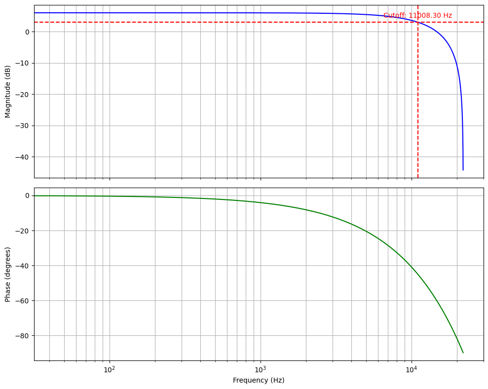
The current cutoff frequency is around 11 kHz. The frequencies up to the cutoff are allowed to pass, but those after are not. The cutoff being nearly the middle of the frequency spectrum is not a coincidence. We chose to place the zero at the maximum frequency and haven't placed any poles or zeros on the frequencies from 0 Hz to 11 kHz. We can move the cutoff frequency by placing more zeros and poles.

High-Pass Filter

The same logic applies to the high-pass filter design as well. We want to have our zero on lowest frequency (which is $z = 1$). We need to place a pole at $z = 0$ to make sure our system is causal. Instead of calculating from scratch, I'll use Python to calculate $a$ and $b$ coefficients from zeros and poles and plot the Bode plot.

from scipy import signal

zeros = [1.0]
poles = [0.0]

# Find the transfer function coefficients.
b, a = signal.zpk2tf(zeros, poles, k=1.0)
b = np.real(b)  # b: [1.0, -1.0]
a = np.real(a)  # a: [1.0, 0.0]

# Calculate the frequency response. 
w, h = signal.freqz(b, a)

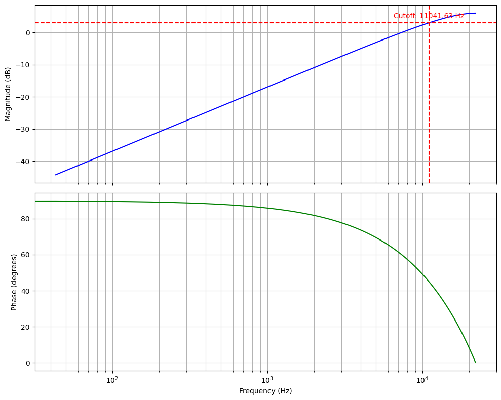
You can see that the lowest frequencies start from -40dB, and we can see half of the maximum power on 11kHz again.

Amplifier

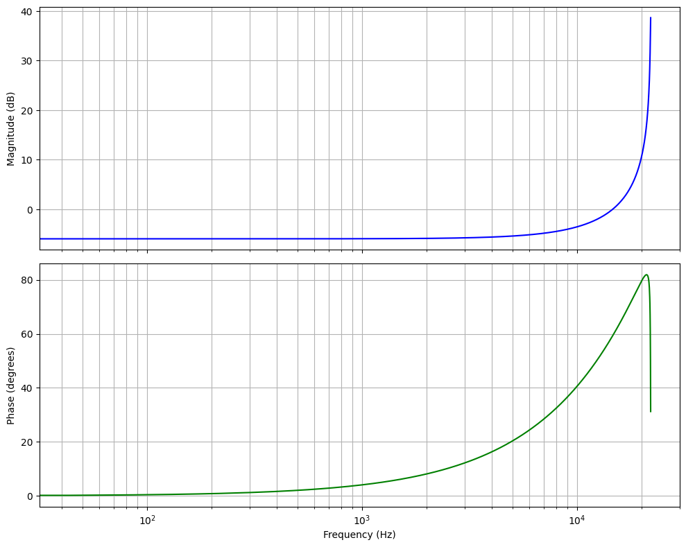
An amplifier is a signal grower in a particular frequency range. It is the opposite of a high/low-pass filter. A high-pass amplifier is going to resonate the highest frequencies. It is being made by adding a pole to the highest frequency ($z = -1$). Please remember that if we place a pole in the unit circle and beyond, we'll have an unstable filter. Therefore, in an amplifier, a pole needs to be close to the unit circle but not on it. I'm choosing $z = -0.99$ for the pole.

from scipy import signal

zeros = [0.0]
poles = [-0.99]

# Find the transfer function coefficients.
b, a = signal.zpk2tf(zeros, poles, k=1.0)
b = np.real(b)  # b: [1.0, 0.0]
a = np.real(a)  # a: [1.0, 0.99]

# Calculate the frequency response. 
w, h = signal.freqz(b, a)

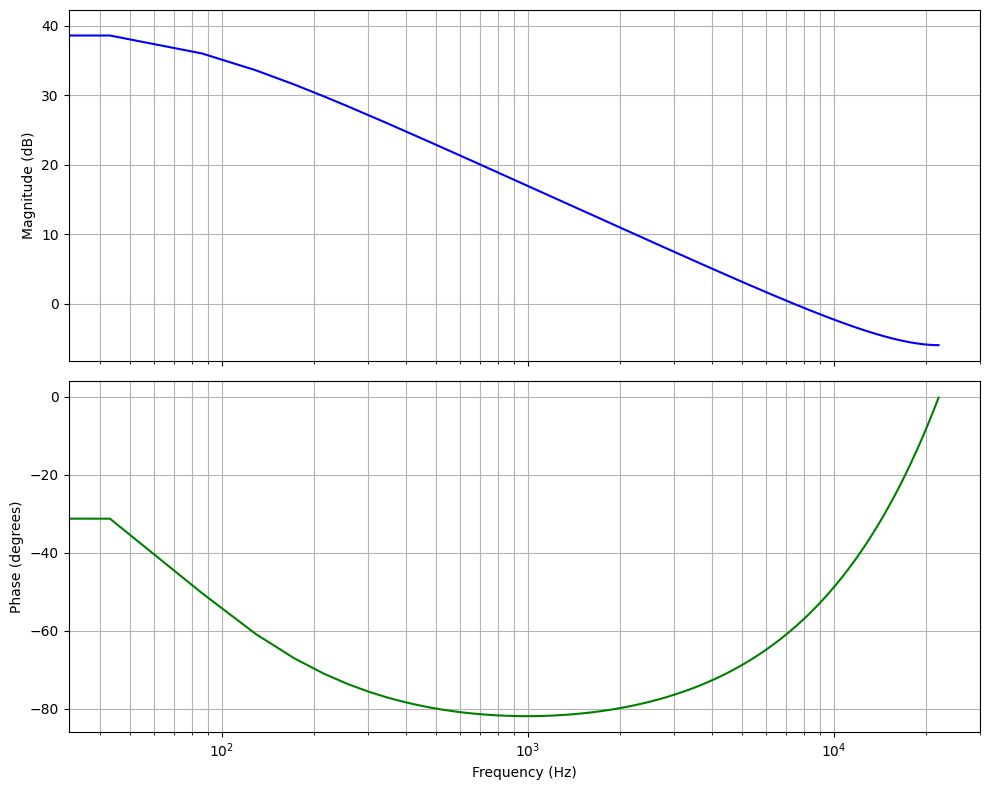
A low-pass amplifier is a filter that amplifies the magnitude of low frequencies. This time, we should set our pole close to $z \approx 1$.

from scipy import signal

zeros = [0.0]
poles = [0.99]

# Find the transfer function coefficients.
b, a = signal.zpk2tf(zeros, poles, k=1.0)
b = np.real(b)  # b: [1.0, 0.0]
a = np.real(a)  # a: [1.0, -0.99]

# Calculate the frequency response. 
w, h = signal.freqz(b, a)

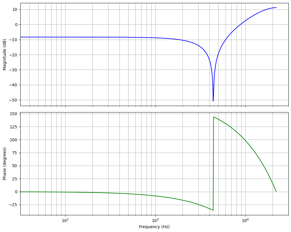
Notch Filter

Some applications require us to have a notch in the magnitude plot of the frequency spectrum. It is particularly useful to remove particular frequencies from our output, like a noise remover. It is actually a zero in a unit circle for a frequency. Imagine it as if we're placing a zero not on the edges of the spectrum like we did for high-pass or low-pass, but for a specific frequency.

Let's design a system that will reduce the response to 4.4 kHz. First of all, we need to find the zero from the frequency. I'll assume the sampling rate as 44.1 kHz.

$$
\omega = 2 \cdot \pi \frac{4400}{44100} \approx \frac{\pi}{5}
$$

We can find the z value by substituting the $\omega$ and using $r = 1$.

$$
z = r \cdot e^{j \omega} = 1 \cdot e^{j \frac{\pi}{5}} = e^{j \frac{\pi}{5}}
$$

As one can understand from the z value, it is a complex variable. However, in real life, it is not possible to have complex coefficients in our transfer function. Therefore, we need to add the complex conjugate pair of the calculated zero to express the transfer function in real coefficients.

from scipy import signal

# Set zeros and poles. Make sure to have complex conjugates in zeros
# to resolve to real values.
zeros = [
    1.0 * np.exp(1j * np.pi / 5),
    1.0 * np.exp(-1j * np.pi / 5),
]
poles = [0.0, 0.0]

# Calculate the transfer function.
b, a = signal.zpk2tf(zeros, poles, k=1.0)
b = np.real(b) # b: [1.0, -1.618, 1.0]
a = np.real(a) # a: [1.0, 0.0, 0.0]

show_filter_response(b, a)

We can apply the same logic by creating a pole instead of a zero to present a notch amplifier.

from scipy import signal

# Set zeros and poles. Make sure to have complex conjugates in poles
# to resolve to real values.
zeros = [0.0, 0.0]
poles = [
    1.0 * np.exp(1j * np.pi / 5),
    1.0 * np.exp(-1j * np.pi / 5),
]

# Calculate the transfer function.
b, a = signal.zpk2tf(zeros, poles, k=1.0)
b = np.real(b) # b: [1.0, 0.0, 0.0]
a = np.real(a) # a: [1.0, -1.618, 1.0]

show_filter_response(b, a)

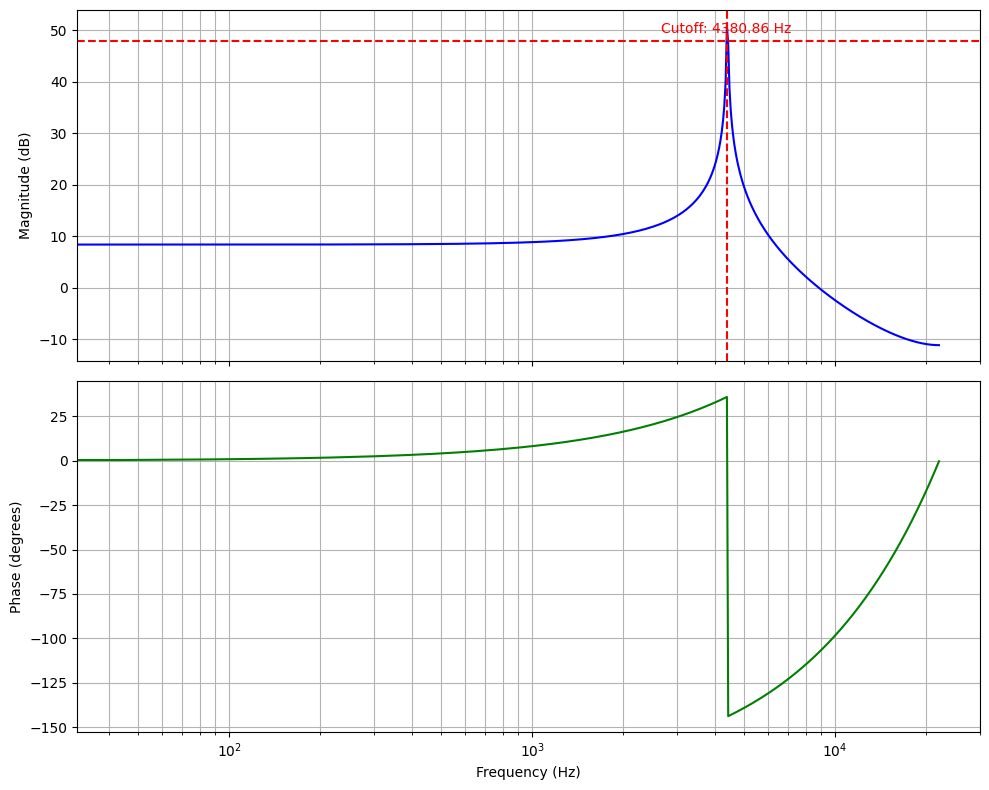
I presented the cutoff frequency in the figure above. Although it shows the -3dB point, the purpose of drawing it is to show you on what frequency we achieved the notch.

Bandpass Filter

A bandpass filter allows the system to pass only a frequency range between two cutoff frequencies. Based on our previous examples, it is a cascaded system that has a high-pass filter with cutoff frequency $f_{c1}$ and a low-pass filter with cutoff frequency $f_{c2}$ where $f_{c2} > f_{c1}$.

By experimenting with the most basic bandpass filter, we can set the zeros on both ends of the frequency spectrum: a zero on $z=1$ for low frequencies and a zero on $z=-1$ for high frequencies.

from scipy import signal

# Set zeros and poles. Make sure to have complex conjugates in poles
# to resolve to real values.
zeros = [1.0, -1.0]
poles = [0.0, 0.0]

# Calculate the transfer function.
b, a = signal.zpk2tf(zeros, poles, k=1.0)
b = np.real(b) # b: [1.0, 0.0, -1.0]
a = np.real(a) # a: [1.0, 0.0, 0.0]

show_filter_response(b, a)

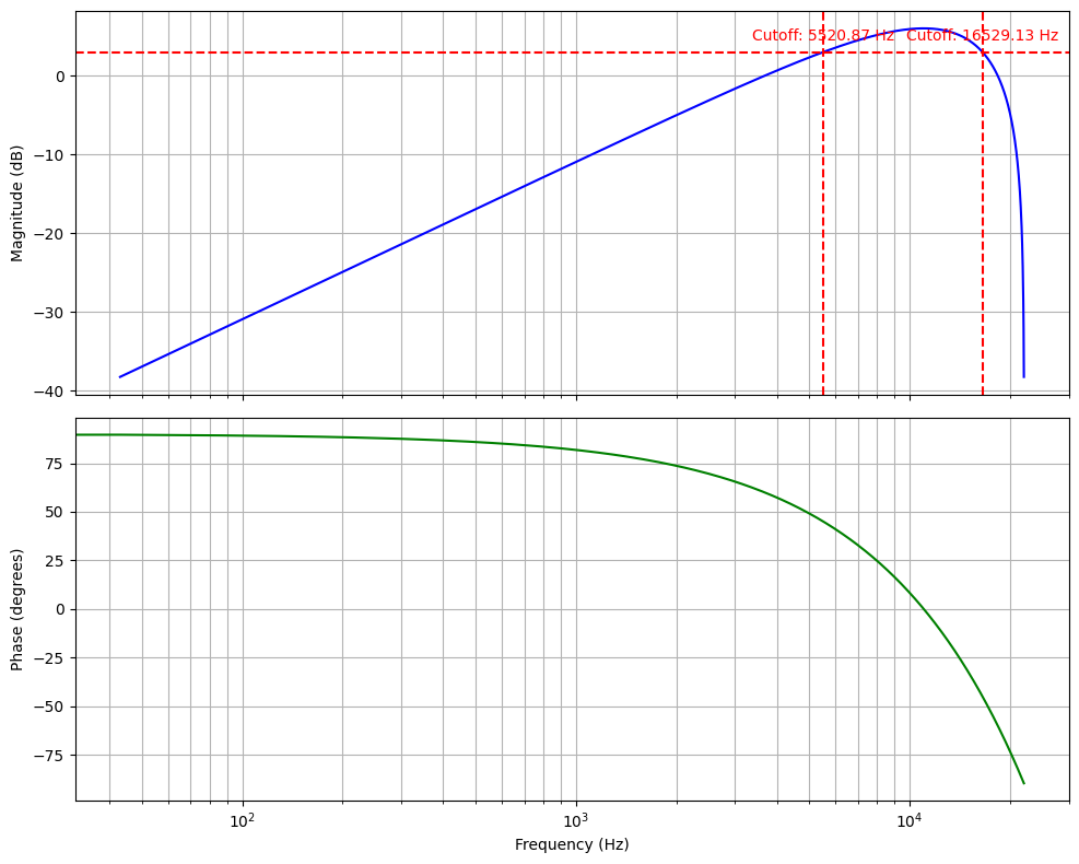
As you can see, the frequency spectrum is divided into two splits. The first low-frequency split ranges from 0 Hz to 11 kHz. Our zero on $z = 1$ placed the cutoff to its middle frequency, $f_{c1} \approx 5500$ Hz. The second half frequency split ranges from 11 kHz to 22 kHz. The other zero placed the cutoff to its middle frequency, again, $f_{c1} \approx 16500$ Hz.

However, the shape of the bandpass filter is not as straight as we expect it to be from the textbook figures. The reason behind it is the lack of poles that will amplify the cutoffs to make the top end like a straight line. Let's make another bandpass filter that uses poles to define a better range of frequencies to pass, and a better uniform magnitude shape on passing frequencies.

The objective is to design a bandpass filter that allows signals between 2.2 kHz and 4.4 kHz to pass. First of all, we'll have a low-pass filter and a high-pass filter with $z=1$ and $z=-1$. This will reduce the magnitudes of signals on both ends of the frequency spectrum. Then, we need to have notch amplifiers on the frequencies we want them to pass.

For frequency 4.4 kHz, we already calculated the z value as $z_1 = e^{j \frac{\pi}{5}}$. We're also going to have its complex conjugate to result in a real-valued transfer function, $z_2 = e^{-j \frac{\pi}{5}}$. For frequency 2.2 kHz, the z value can be calculated as the following equation. We will have the complex conjugate of the $z_3$ as $z_4$.

$$
z_3 = r \cdot e^{j\omega} = r \cdot e^{j \cdot 2 \pi \frac{f}{f_{sr}}} = 0.90 \cdot e^{j \cdot 2 \ pi 2200 / 44100} = e^{j \ pi / 10}
$$

Please notice that I selected $r = 0.90$. It is based on my experiences with how high peaks I want to have. With a value of 0.99, the peaks were so high that a straight shape wasn't possible. I see that 0.85 to 0.90 values are feasible.

Therefore, in the end, we can use the following Python script to calculate the $a$ and $b$ coefficients and plot the frequency response.

from scipy import signal

# Set zeros and poles. Make sure to have complex conjugates in poles
# to resolve to real values.
zeros = [1.0, -1.0]
poles = [
    0.90 * np.exp(1j * np.pi / 10),
    0.90 * np.exp(-1j * np.pi / 10),
    0.90 * np.exp(1j * np.pi / 5),
    0.90 * np.exp(-1j * np.pi / 5)
]

b, a = signal.zpk2tf(zeros, poles, k=1.0)
b = np.real(b)
a = np.real(a)

show_filter_response(b, a)

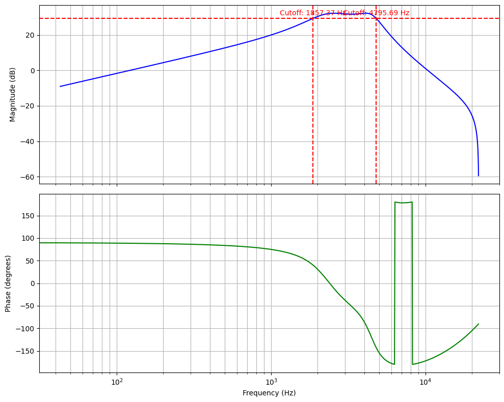
In the figure above, you can see that we have nearly a perfect bandpass filter whose cutoffs are defined as $f_{c1} = 1.9$ kHz and $f_{c2} = 4.8$ kHz.

Last Words and Discussions

Up to this section, I tried to explain how digital signal processing works and what the procedure is to design simple digital filters manually. There are better methods, of course, or better teachers, but I believe this guide will be a great getting-started guide for the people who are afraid of starting to learn this magnificent topic.

Thanks again to everyone for reading it up to now. In the era of artificial intelligence, it was a great opportunity for me to write what I learned without any help from LLM models. I'm going to suggest that everyone follow the path of DSP by understanding how to go from cutoff frequencies to filters instead of the other way around. There's a method called Bilinear Transformation, which helps you to do it. Then, the next stop should be popular filters like Butterworth and Chebyshev.

I'm trying to develop a DSP library in Mojo language, as I said earlier, you can also check the library out to see how one can implement these algorithms we discussed in the computational domain.

GitHub - electricalgorithm/dsplib-mojo: An introduction to digital signal processing with Mojo language.

An introduction to digital signal processing with Mojo language. - electricalgorithm/dsplib-mojo

GitHubelectricalgorithm

Have fun!

Feel free to contact me for any typos, mistakes or questions: [email protected]

Appendix

Appendix A1. Interactive Bode Plot in Python

I'm using the following Python code block to generate the graphs to make them interactive.

import numpy as np
import matplotlib.pyplot as plt
from scipy import signal

import numpy as np
import matplotlib.pyplot as plt

import plotly.graph_objects as go
from plotly.subplots import make_subplots


def plot_bode_interactive(w, h, fs=44100, y_axis_limits=[-60, 10]):
    freq_hz = (w * fs) / (2 * np.pi)
    # Using a floor of 1e-12 to prevent math errors, though the plot range will hide this
    magnitude_db = 20 * np.log10(np.abs(h) + 1e-12)
    phase_deg = np.angle(h, deg=True)

    fig = make_subplots(rows=2, cols=1,
                        shared_xaxes=True,
                        vertical_spacing=0.1,
                        subplot_titles=("Magnitude Response", "Phase Response"))

    # Magnitude Trace
    fig.add_trace(
        go.Scatter(x=freq_hz, y=magnitude_db, name="Magnitude",
                   line=dict(color='#1f77b4', width=2),
                   hovertemplate='<b>Freq</b>: %{x:.2f} Hz<br><b>Mag</b>: %{y:.2f} dB<extra></extra>'),
        row=1, col=1
    )

    # Fixed -3dB line to show half power point.
    fig.add_hline(y=-3, line_dash="dot", line_color="red", opacity=0.5, row=1, col=1)

    # Phase Trace
    fig.add_trace(
        go.Scatter(x=freq_hz, y=phase_deg, name="Phase",
                   line=dict(color='#2ca02c', width=2),
                   hovertemplate='<b>Freq</b>: %{x:.2f} Hz<br><b>Phase</b>: %{y:.2f}°<extra></extra>'),
        row=2, col=1
    )

    # Limit X-axis to standard range (20Hz to Nyquist)
    fig.update_xaxes(type="log", range=[np.log10(20), np.log10(fs/2)],
                     title_text="Frequency (Hz)", gridcolor='lightgray')

    # Limit Y-axis so we don't see the floors
    # This keeps the focus on the passband and the transition
    fig.update_yaxes(range=y_axis_limits, title_text="Magnitude (dB)", row=1, col=1, gridcolor='lightgray')

    fig.update_yaxes(title_text="Phase (degrees)", row=2, col=1, gridcolor='lightgray')

    fig.update_layout(
        height=800,
        template="plotly_white",
        showlegend=False,
        hovermode="x unified"
    )
    fig.show()